Hunting for Exoplanets
A team of exoplanet searchers recently released a large set of data. The goal of this article is to review one method of finding exoplanets, and then to apply those methods to the released data.
Background
When solving for planetary orbits, most students are told to make the simplifying assumption that the star is infinitely massive. However, the star really does have finite mass and mutually orbits its planets. This motion would appear to the observer as a periodic wobble in the velocity of the star. We should be able to detect this stellar wobble, and thus infer the existence of an exoplanet.
Systemic
Systemic Console 2 is a tool for analyzing stellar velocity data for the presence of exoplanets. It comes pre-loaded with radial velocity data from many sources. There is a 4 part tutorial on using the software. Though it is written for an older version, the core features are the same.
Unfortunately, I ran into several problems trying to get Systemic Console 2 to work properly. On my Mac laptop, I ran into a launch time problem, and found the corresponding github issue. I then installed an Ubunutu 16.04 virtual machine and attempted to run the software in that environment. The results were more promising (the application opened), but ultimately unsuccessful. A quick search revealed that I am not alone and that an issue had already been reported.
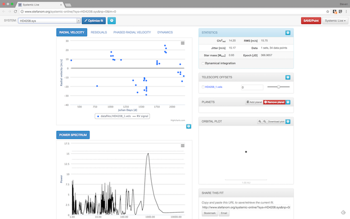
Fortunately, there is also a web-based version of Systemic called Systemic Live. I can load the HD 4208 data into the program just like in the tutorial.

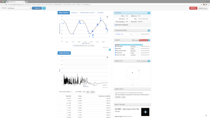
Manually adjusting the parameters and then applying the optimization yields the following fit.

With a χ2 = 2.52, the fit here isn’t as good as the one in the desktop version of the tutorial. Starting from different manual adjustments reaches different fits, but this was the best one I achieved.
Manually fitting the data
Since I couldn’t get Systemic Console to work properly and Systemic Live doesn’t allow data sets to be uploaded, I made an attempt to write my own curve-fitting techniques. We will take a look at the same star as above, HD 4208. First, we inspect the data file from the Keck data set.
2451010.10523     17.69   1.20  0.1653 -1.00000    118398   275
2451014.09906     16.36   1.57  0.1549 -1.00000    108803   220
2451043.04968     17.16   1.36  0.1620 -1.00000    153146   300
2451044.03377     14.95   1.54  0.1695 -1.00000    123400   250
2451068.93885     17.62   1.45  0.1666 -1.00000    112870   350
2451172.74280     11.17   1.21  0.1724 -1.00000    103587   330
2451368.07957    -11.41   1.33  0.1621 -1.00000     83174   170
2451412.06450     -9.44   1.43  0.1679 -1.00000     81332   200
2451543.73889    -16.59   1.42  0.1603 -1.00000     70334   300
2451550.72615    -13.45   1.38  0.1653 -1.00000     70202   246
2451551.71323    -15.73   1.38  0.1610 -1.00000     62811   300
2451552.71126    -19.21   1.29  0.1614 -1.00000     76306   400
2451580.70569    -15.87   1.52  0.1592 -1.00000     69841   240
2451581.70668    -20.39   1.50  0.1615 -1.00000     54075   220
2451582.72443    -22.11   1.49  0.1784 -1.00000     53935   210
2451583.70664    -18.30   1.58  0.1711 -1.00000     54115   240
2451585.70754    -15.08   1.58  0.1708 -1.00000     51083   300
2451755.03303     14.05   1.28  0.1882 -1.00000     88457   500
2451756.02566      9.54   1.38  0.1874 -1.00000     82038   500
2451757.07363     10.84   1.24  0.1723 -1.00000     92138   500
2451793.93004      9.57   1.45  0.1871 -1.00000     68418   241
2451882.72859     21.83   1.28  0.1563 -1.00000     77493   240
2451883.77274     20.19   1.41  0.1628 -1.00000     76855   248
2451899.77756     21.60   1.11  0.1661 -1.00000     99607   421
2451900.74929     14.63   1.30  0.1603 -1.00000     93264   258
2452095.11183      3.92   1.68  0.1309 -1.00000     98288   273
2452129.09608      0.00   1.46  0.1450 -1.00000     84005   197
2452133.04676     -4.75   1.49  0.1405 -1.00000     76686   145
2452134.00916     -4.97   1.43  0.1477 -1.00000     81811   150
2452161.92847    -10.02   1.56  0.1499 -1.00000     81097   176
2452187.98133     -8.49   1.48  0.1476 -1.00000     80402   475
2452489.03795     -2.16   1.64  0.1509 -1.00000     91243   148
2452538.89542      4.94   1.67  0.1498 -1.00000     97016   161
2452601.80071      8.16   1.49  0.1534 -1.00000    111846   275
2452833.08079     15.11   1.62  0.1401 -1.00000     97009   166
2453196.07518    -20.63   1.72  0.1428 -1.00000     98598   150
2453604.08199     17.84   1.39  0.1432  0.03119    103305   184
2454464.81619      7.83   1.41  0.1699  0.03083     71875     0
2455169.84484      9.33   1.39  0.1672  0.03125     50867   141
2455169.84730      5.34   1.36  0.1637  0.03127     47470   136
2455467.04618    -18.28   1.36  0.1535  0.03115     49407   107
2455807.09469    -17.88   1.52  0.1485  0.03123     49077   152
2456138.13949      0.95   1.38  0.1489  0.03102     47374    81
2456513.13532    -39.46   1.59  0.1578  0.03112     49372    80
2456613.86212    -24.23   1.32  0.1578  0.03134     48670    92
2456638.73076    -15.93   1.46  0.1592  0.03126     50469   121
2456874.13410     -1.28   1.51  0.1509  0.03106     48822   101
2456907.08927     -0.43   1.59  0.1567  0.03121     49106    93
The first column is the Julian Date. The second column is the measured velocity in m/s. The third column is the uncertainty in the velocity, also in m/s. The fourth column is the S_value and the fifth column is H_alpha. The fifth column is the median number of photons per pixel, and the fifth column is the exposure time in seconds.
References and Links
- Butler, Vogt, Laughlin, et al., The LCES HIRES/KECK Precision Radial Velocity Exoplanet Survey (2017) Link
- Data release
- Systemic Console homepage
- Systemic Console on Github
- 4 part Systemic Console Tutorial