Fitting Cosmic Ray Data

Introduction

Cosmic Rays

Cosmic rays are very high energy particles with deep space origins that are detected on Earth. Generally, only massive particles are considered cosmic rays. We know that they originate in outer space, because their intensity increases with altitude. Furthermore, we know that most cosmic rays are charged particles, because the intensity differs by latitude, suggesting that they are being deflected by Earth’s magnetic field.

Primary cosmic rays are those that arrive from space. Sometimes the primary cosmic rays will collide with particles in the atmosphere and produce a cascade of secondary cosmic ray particles.

The dataset analyzed on this page is from a balloon experiment that detected primary cosmic rays.

Cosmic Ray Data

To analyze the cosmic ray data, I will use Python with the pandas, numpy, and matplotlib libraries. We will import the following libraries for use in the code below

import pandas as pd
import numpy as np
import matplotlib.pyplot as plt

Then we can import the data file as a pandas DataFrame

df = pd.read_table('cosmicrays.dat', sep='\s+')

To inspect the data we can use

print(df.head())

which gives

    Event   Primary   E,TeV
  0    A-52    Fe      1.4 
  1    B-146   Fe      1.4 
  2    D-1-9   C      10.1 
  3    D-1-27  Ca      8.9 
  4    D-1-34  Cl     18.6 

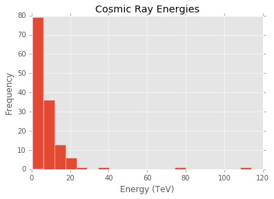
It can also be useful to look at a histogram of energies. We can generate this with the following

matplotlib.style.use('ggplot')

plt.figure()
df['E,TeV'].plot(kind='hist', title='Cosmic Ray Energies', bins=20)
plt.xlabel('Energy (TeV)')

which yields

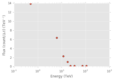
Many cosmic ray spectra plot differential flux of particles on the y-axis. We can get this from our data by binning the energies. Our flux proxy is then given by dividing the count of detections within the energy bin by the size of the energy bin. The plot of particle flux versus particle energy is shown below.

That plot was generated with

hist, bins = np.histogram(df['E,TeV'], bins=20)
deltaE = np.diff(bins)

flux = hist / deltaE
flux[flux == 0] = np.nan

fig = plt.figure()
ax = plt.gca()
ax.plot(bins[:-1], flux, 'o')
ax.set_xscale('log')
plt.xlabel('Energy (TeV)')
plt.ylabel('Flux (count/$\Delta E$) (TeV$^{-1}$)')

In the code above, we set the 0 fluxes to nan to prevent them from being plotted. The idea here is that these 0 fluxes are due to the sparseness of our data and choice of bin, rather than any real effect.

Fitting the Data

We can try to get an expression for the particle flux by fitting a curve to our data above. According to the Particle Data Group, the intensity generally fits a power law. We can use the curve fitting capability of scipy to get a curve fit. First we need to import the curve fit function and then define our test function.

from scipy.optimize import curve_fit

def func(x, a, b):
    return a*(x**b)

and sanitize our data

bin_mid_clean = bin_mid[~np.isnan(flux)]
flux_clean = flux[~np.isnan(flux)]

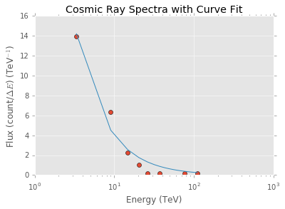
Then we can use the function to get best fit coefficients and correlations, and then plot the fitted curve along with our original data.

coeff, corr = curve_fit(func, bin_mid_clean, flux_clean)

plt.figure()
ax = plt.gca()

ax.plot(bin_mid, flux, 'o', label='Original Data')
ax.set_xscale('log')

plt.xlabel('Energy (TeV)')
plt.ylabel('Flux (count/$\Delta E$) (TeV$^{-1}$)')
plt.title('Cosmic Ray Spectra with Curve Fit')
plt.plot(bin_mid, func(bin_mid, *coeff), label='Fitted Line')

which yields the graph

and the fitted curve of

$$ \frac{dN}{dE} = 57.12 (\frac{E}{1 \textrm{TeV}})^{-1.15} $$

Concluding Remarks

There is speculation about a `knee’ in the energy spectrum at around 10^15 eV. This data set does not contain enough detections at high energies to make a conclusion.

Bibliography

Carroll, Bradley W. and Ostlie, Dale A., An Introduction to Modern Astrophysics, 2nd Ed., Pearson Education, Inc. (2007)

C. Patrignani et al. (Particle Data Group), Chin. Phys. C, 40, 100001 (2016)

Wolchover, Natalie, The Particle That Broke a Cosmic Speed Limit, Article Link (2015)